Kalman Filter
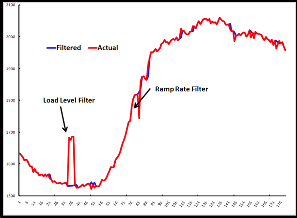
The Kalman Filter smooths through data anomalies as they flow in from the raw meter data. The Kalman Filter uses a two-stage filter when both a Level and Ramp Rate Model are defined. The first filter compares observed ramp rates to expected ramp rates from the selected ramp rate model. Observed ramp rates that are outside of a user specified tolerance are marked as Bad and excluded from further calculations. The ramp rate filter will capture random spikes (upward and downward) in loads. The second filter compares observed loads to expected loads from the selected level model. Observed loads that are outside of a user specified tolerance are marked as Bad and excluded from further calculations. An observed load that satisfies both the ramp rate filter and the load level filter is accepted as a valid data point. The type of data anomalies that will be captured by these two filters are depicted below.
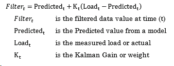
The basic idea behind a Kalman Filter assumes that load data is measured with error. The larger the measurement error the less certain we are that the current metered value is a true representation of the demand for energy. In this case it makes sense to rely on an estimated value rather than the metered value. Of course, the smaller the measurement error the more reliant we want to be on that data. A Kalman Filter creates a filtered value which is a weighted average of the observed data and a predicted value. The more precise the measurement the greater the weight is placed on the observed data. This idea can be written mathematically as follows:
The Kalman Gain is computed as:
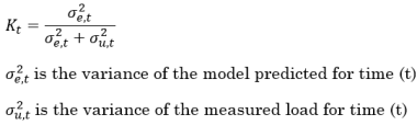
In this case, the more precise the load measurement the smaller will be the measurement variance, and hence the greater the weight, K, that is placed on the actual value. Conversely, measurement imprecision leads to a greater reliance on the model predicted. Another way to think about the Kalman Filter is that the "noisier" the actual data are the more we want to rely on the result from a model which is averaging through the noise. With a heavy reliance on autoregressive terms in the forecast models it is important that the "noise" in the actual load be removed to prevent forecast instability
The Kalman Filter as described above will always replace the actual load value with a filtered value. In load forecasting there are many times when we want the load forecast models to launch off the actual and not filtered load. For example, during the morning ramp up it is important that the models forecast off the end of the most recent actual. To achieve this, we need an ability to switch the Kalman Filter on and off. In mathematical terms we need a way to set the Kalman Weight to 1.0 when we want to use the actual load and to a value of 0.0 when the load is an outlier. This leads to a Two Stage Modified Kalman Filter that is available in MetrixIDR.
Stage One – Ramp Rate Filter. The first stage of the Two Stage Kalman Filter compares the observed ramp rate to an expected ramp rate. If the observed ramp rate is significantly different from the expected ramp rate there is an indication that the current load value is a spike (either upward or downward). This implies the binary filter described below.
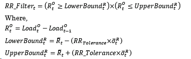
Here, the Ramp Rate filter is a binary variable that returns a value of 1.0 if the observed ramp rate in period (t) is between the expected bounds for the ramp rate and 0.0 otherwise. The bounds are computed as the expected ramp rate  +/- the user defined Ramp Rate tolerance times the standard deviation around the expected ramp rate
  . The value for the expected ramp rate and its standard deviation are derived from the user selected Kalman Filter Model. The Ramp Rate tolerance and Kalman Filter Model are set by the user as part of the Manage TOU Parameter Sets (KF Std Err Up and KF Std Err Down parameters).
Stage Two – Level Filter. The second stage of the Two Stage Kalman Filter compares the observed load level to an expected load level. It is intended to capture load shifts. If the observed load is significantly different from the expected load there is an indication of a load shift. This implies the binary filter described below.
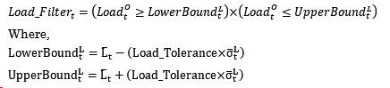
Here, the Load filter is a binary variable that returns a value of 1.0 if the observed load level in time period (t) is between the expected bounds for the load and 0.0 otherwise. The bounds are computed as the expected Load  +/- the user defined Load tolerance times the standard deviation around the expected load
  . The value for the expected load level and its standard deviation are derived from the user selected Kalman Model. The Load tolerance and the Kalman Model are set by the user as part of the Kalman Filter Options.
Kalman Filter. Given the values for the First and Second Stage filters the final Kalman Filter can be written as follows.
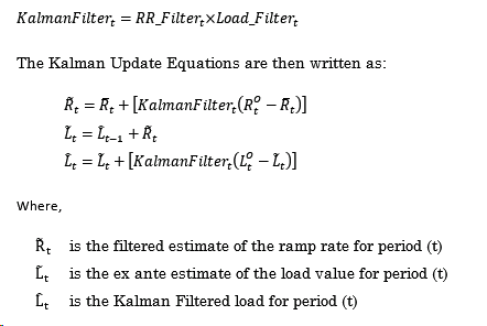
In the case where the current load value satisfies both the Ramp Rate and Load Filters, then  will be equal to the observed load. In the case where either the Ramp Rate or the Load Filter, or both fail the observed load value is marked as Bad and is excluded from further calculations.