Model Estimation

If the user enters a scale elasticity adjustment factor other than 1.0, the end-use model inputs are recomputed with k*Elas used as the elasticity all each scale drivers in all sectors. This calculation is performed local to the model calculations and is not visible in the SAE Sets module. The idea is as follows.

To allow regional economic values to be used for sub regional models, a final scale elasticity adjustment is entered at the model level. This adjustment is only available when the SAE approach is selected. The adjustment can be edited on the Energy, Peak, or HLH model properties dialogs.

The idea behind the adjustment is that the area being modeled may grow faster or slower than the regional economic data being used in the SAE Set. The user could always duplicate the SAE set and enter lower elasticities. But the scale elasticity adjustment offers a simpler approach that allows the user to dampen or amplify this elasticity, as appropriate.

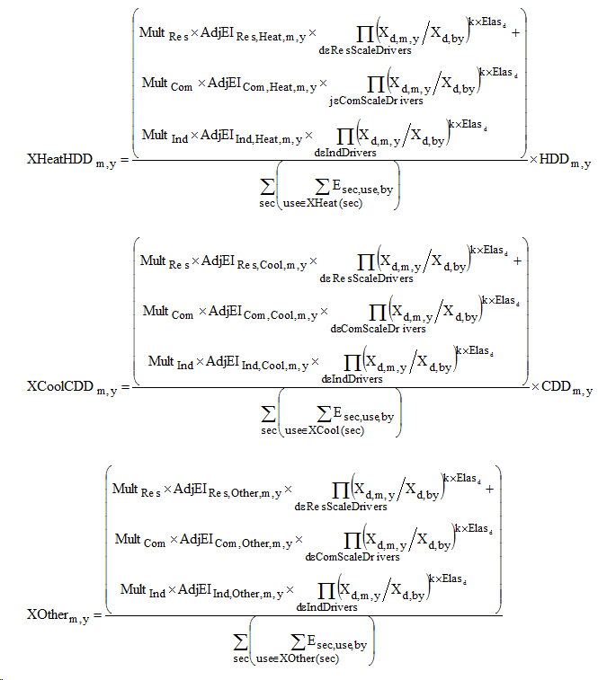
The elasticity adjustment is introduced in the construction of the final variables that are used in the SAE model statistical step. In this step, a regression model is estimated using the Y variable constructed using the Add Back method for new technologies, and X variables constructed using the SAE calculations with the elasticity modifier applied to all of the rate-class sector elasticities. The final equation for the SAE model X variables are as follows. In these equations, the parameter (k) is the scale elasticity adjustment factor. The user can directly edit this adjustment on the model forms.

To provide the user with an idea about the elasticity a Calculate button is provided on the Energy Tab of the Model Specification dialog. This button uses the data to detect the apparent elasticity and provides the result to the user. The user can then decide about the value to use (or maybe whether to modify the drivers or driver elasticities directly). The logic of the calculation is as follows:

• Step 1: Estimate a exploratory regression of Monthly Energy on the SAE variables (XHeat * HDD, XCool * CDD, XOther). If there are multiple HDD or CDD variables then include all corresponding XHeat and XCool interaction variables in the regression. This exploratory regression will include a constant term.
• Step 2: Compute average values. Compute the average value for Monthly Energy and each of the explanatory variables. These averages will be used in the elasticity calculations.
• Step 3: Compute elasticities. Use the regression coefficients from step 1 and the average values from step 2 to compute elasticities at the mean value for each of the explanatory variables.

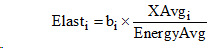
where bi is the slope on the ith explanatory variable from the regression, XAvgi is the average X value in the estimation period, and EnergyAvg is the average of the monthly energy values in the estimation period.

• Step 4: Sum the elasticities across the explanatory variables.

The resulting sum is presented to the user, who can then modify the elasticity adjustments for Energy, Peak, and HLH if desired.